Examine This Report about Vlookup Excel

By pressing ctrl+change+facility, this will calculate and also return worth from numerous ranges, as opposed to simply individual cells added to or increased by each other. Calculating the sum, item, or quotient of individual cells is very easy-- simply utilize the =AMOUNT formula and enter the cells, values, or array of cells you intend to do that arithmetic on.

If you're looking to find total sales income from several marketed devices, for instance, the range formula in Excel is excellent for you. Here's just how you 'd do it: To begin making use of the selection formula, type "=AMOUNT," and also in parentheses, go into the very first of 2 (or three, or 4) varieties of cells you 'd like to increase together.

This represents multiplication. Following this asterisk, enter your 2nd series of cells. You'll be multiplying this 2nd array of cells by the very first. Your progression in this formula should currently appear like this: =AMOUNT(C 2: C 5 * D 2:D 5) Ready to press Get in? Not so quick ... Because this formula is so difficult, Excel books a various keyboard command for arrays.

This will acknowledge your formula as an array, covering your formula in brace personalities and effectively returning your product of both varieties integrated. In profits computations, this can lower your time and also initiative substantially. See the last formula in the screenshot over. The COUNT formula in Excel is denoted =COUNT(Beginning Cell: End Cell).

For instance, if there are eight cells with gone into values between A 1 as well as A 10, =MATTER(A 1: A 10) will return a worth of 8. The COUNT formula in Excel is particularly useful for large spreadsheets, wherein you want to see the amount of cells contain real entries. Don't be deceived: This formula won't do any math on the values of the cells themselves.

Examine This Report on Excel Shortcuts

Making use of the formula in bold over, you can quickly run a count of current cells in your spreadsheet. The outcome will look a something such as this: To do the ordinary formula in Excel, enter the values, cells, or array of cells of which you're determining the standard in the layout, =STANDARD(number 1, number 2, and so on) or =STANDARD(Beginning Worth: End Worth).

Discovering the average of a variety of cells in Excel keeps you from having to find individual sums and also after that doing a different division equation on your total. Making use of =STANDARD as your first message entrance, you can allow Excel do all the benefit you. For recommendation, the average of a team of numbers is equal to the amount of those numbers, split by the number of products in that group.

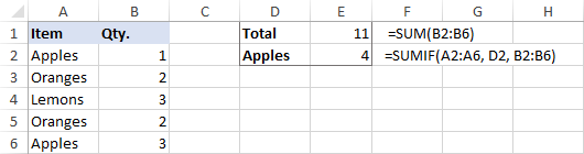
This will return the amount of the worths within a desired array of cells that all satisfy one standard. For instance, =SUMIF(C 3: C 12,"> 70,000") would certainly return the sum of values between cells C 3 as well as C 12 from just the cells that are higher than 70,000. Let's claim you intend to establish the profit you produced from a checklist of leads who are linked with specific area codes, or calculate the sum of particular staff members' incomes-- yet just if they fall above a specific quantity.

With the SUMIF function, it doesn't need to be-- you can easily build up the sum of cells that fulfill particular standards, like in the income example over. The formula: =SUMIF(range, requirements, [sum_range] Variety: The array that is being evaluated using your requirements. Requirements: The criteria that identify which cells in Criteria_range 1 will certainly be added together [Sum_range]: An optional array of cells you're mosting likely to include up along with the first Range went into.

In the instance listed below, we desired to determine the sum of the salaries that were greater than $70,000. The SUMIF feature added up the dollar amounts that went beyond that number in the cells C 3 with C 12, with the formula =SUMIF(C 3: C 12,"> 70,000"). The TRIM formula in Excel is signified =TRIM(message).

How Learn Excel can Save You Time, Stress, and Money.

For instance, if A 2 includes the name" Steve Peterson" with undesirable areas prior to the initial name, =TRIM(A 2) would return "Steve Peterson" with no spaces in a new cell. Email and submit sharing are fantastic tools in today's office. That is, up until among your coworkers sends you a worksheet with some truly funky spacing.

As opposed to fastidiously eliminating as well as including spaces as required, you can tidy up any kind of irregular spacing making use of the TRIM function, which is used to remove added rooms from information (besides solitary spaces in between words). The formula: =TRIM(message). Text: The text or cell where you intend to get rid of rooms.

To do so, we entered =TRIM("A 2") into the Solution Bar, as well as replicated this for every name below it in a brand-new column next to the column with undesirable spaces. Below are a few other Excel solutions you might discover valuable as your data administration requires grow. Allow's say you have a line of message within a cell that you wish to break down right into a few different sectors.

Purpose: Utilized to remove the very first X numbers or personalities in a cell. The formula: =LEFT(message, number_of_characters) Text: The string that you wish to extract from. Number_of_characters: The number of personalities that you desire to extract beginning with the left-most personality. In the instance listed below, we got in =LEFT(A 2,4) right into cell B 2, and replicated it into B 3: B 6.

Purpose: Made use of to remove characters or numbers between based upon setting. The formula: =MID(text, start_position, number_of_characters) Text: The string that you desire to draw out from. Start_position: The setting in the string that you intend to start drawing out from. For instance, the first placement in the string is 1.

Some Known Incorrect Statements About Excel Skills

In this example, we went into =MID(A 2,5,2) right into cell B 2, as well as replicated it into B 3: B 6. That enabled us to remove both numbers starting in the fifth setting of the code. Objective: Utilized to extract the last X numbers or characters in a cell. The formula: =RIGHT(text, number_of_characters) Text: The string that you desire to draw out from.

formulas excel if cell contains text excel formulas don't update excel formulas without functions